Condensed Matter II

Lattice dynamics- starting assumptions

Adiabatic approximation- assume electrons are attached rigidly to the nucleus.
Assume the amplitude of the vibrations is small.
Harmonic approximations- terms of order higher than u² in the interatomic potential are neglected.

One-dimensional monatomic chain: we’ll start by only including nearest neighbour forces.

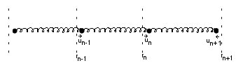
positions r_n, equilibrium atomic separation r_n-r_n-1=a

displacements from equilibrium u_n

Interatomic pair potential $\phi(r_2-r_1)$

Potential energy of nth atom $V_n=\phi(r_{n+1}-r_n)+\phi(r_n-r_{n-1})$

Taylor expansion about r_n-r_n-1=a

$\phi(r_2-r_1)=\phi(a)+(u_2-u_1)\phi' (a)+\frac{1}{2}(u_2-u_1)^2\phi'' (a)+\ldots$

Φ’(a)=0, so $V_n=\frac{1}{2}(u_{n+1}-u_n)^2\phi''(a)+\frac{1}{2}(u_n-u_{n-1})^2\phi''(a)+2\phi(a)$

Force $F=\frac{-\partial V_n}{\partial u_n}$

Also note that Φ’’(a) can be written as the force constant, C.

In fact, having done all that, we could have just started from this point by remembering Hooke’s Law F=Cx (where x is displacement from equilibrium).

$F=m\frac{\partial^2u_n}{\partial t^2}=C\{(u_{n+1}-u_n)-(u_n-u_{n-1})\}$

$m\frac{\partial^2u_n}{\partial t^2}=C\{ u_{n+1}-2u_n+u_{n-1})\}$

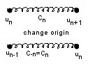
Aside: just to check that we aren’t fiddling our force constants to make everything neat, we can use Newton III to show that C_n=C_-n

If we wanted to include more distant neighbour interactions (up to the Nth), our equation at this point would have the form

$m\frac{\partial^2u_n}{\partial t^2}=\sum_{p=1}^NC_p\{u_{n+p}-2u_n+u_{n-p}\}$

Going back to nearest neighbours, try a solution of the form

$u_n=Ae^{i(kna-\omega t)}$

$u_{n+p}=Ae^{i(k(n+p)a-\omega t)}$

-> $-m\omega^2=C(e^{ika}-2+e^{-ika})$

$-m\omega^2=2C(\cos ka-1)$

$m\omega^2=4C\sin^2\frac{ka}{2}$

$\omega=2\sqrt{\frac{C}{m}}\sin\frac{ka}{2}$

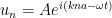
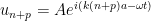
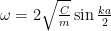
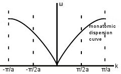
Dispersion relation

Nearest neighbours only

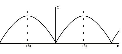
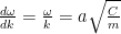
In the long wavelength limit (small k), $\sin\frac{ka}{2}\rightarrow \frac{ka}{2}$

$\omega=a\sqrt{\frac{C}{m}}k$

$\frac{d\omega}{dk}=\frac{\omega}{k}= a\sqrt{\frac{C}{m}}$ speed of sound

Considering more distant neighbours

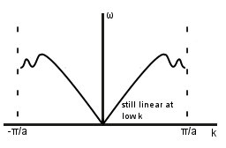
Rule of thumb- number of modulations = number of further neighbour interactions considered.

Brillouin Zones: all the physics of a system is contained within a Brillouin Zone. The standard definition of the BZ is that it is “the Wigner-Seitz unit cell in reciprocal space”, but there’s no point just quoting this if you don’t understand (or can’t readily explain) what it means. For that reason, it also helps to remember this alternate definition-

The first Brillouin Zone is the set of points closer to the origin in reciprocal space than any other reciprocal lattice point.

The nth Brillouin Zone is the set of points reached from the origin in reciprocal space by crossing n-1 Bragg planes and no fewer.

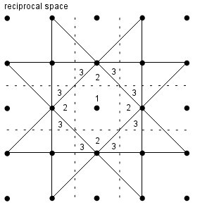
Each Brillouin Zone has the same volume. Any normal mode can be represented by a wavevector in the first Brillouin Zone.

1D diatomic chain- intuitive method

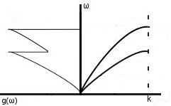
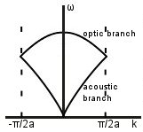
For a diatomic chain, the repeat distance is doubled in real space, so it is halved in k-space (i.e. the size of the Brillouin Zone is halved). At first glance, this seems to mean we have lost the information contained in the $\frac{\pi}{2a}<|k|<\frac{\pi}{a}$ region. If we want to retain it, we will have to translate it back into the new 1^st Brillouin Zone.

If the two types of atom have different masses, a gap opens up between the two branches.

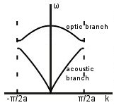
As you’ll see from the graphs, we’ve suddenly introduced the terms acoustic and optic branch, but don’t panic. You didn’t miss anything- these terms will be described below once we go through the maths of the 1D diatomic chain.

1D diatomic chain- the maths: use all the same assumptions as the monatomic chain.

Equation of motion for white atoms $m_1\frac{partial^2u_n}{\partial t^2}=C(u_{n+1}-2u_n+u{n-1})$

Equation of motion for black atoms $m_2\frac{partial^2u_{n-1}}{\partial t^2}=C(u_{n}-2u_{n-1}+u{n-2})$

Try solutions m₁ $u_n=Ae^{i(kna-\omega t)}$

m₂ $u_{n-1}=\alpha Ae^{i(k(n-1)a-\omega t)}$

$-m_1\omega^2=C(\alpha e^{ika}-2+\alpha+e^{-ika})$

$-m_2\omega^2=C(e^{ika}-2\alpha+e^{-ika})$

Eliminating α leads to

$\omega^2=\frac{C(m_1+m_2)}{m_1m_2}\pm C\{\frac(m_1+m_2)(m_1m_2)^2-\frac{4}{m_1m_2}\sin^2ka\}^\frac{1}{2}$

An alternate (and quite neat) method to get this answer without too much trouble is to use matrices as follows.

Start with trial solutions of the form

$u_n=Ae^{i(kna-\omega t)}$

$u_{n-1}=Be^{i(k(n-1)a-\omega t)}$

This gives

$-Am_1\omega^2=2C(B\cos ka-A)$

$-Bm_2\omega^2=2C(A\cos ka-B)$

We can rewrite this in matrix form

$\left[ \begin{array}{cc} 2C-m_1\omega^2&-2C\cos ka \\ -2C\cos ka&2C-m_2\omega^2 \end{array} \right]$ $\left[ \begin{array}{c} A \\ B \end{array} \right] =0$

For non-trivial solutions

$\left| \begin{array}{cc} 2C-m_1\omega^2&-2C\cos ka \\ -2C\cos ka&2C-m_2\omega^2 \end{array} \right|=0$

$(2C-m_1\omega^2)(2C-m_2\omega^2)-4C^2\cos^2 ka=0$

This gives us a quadratic in ω² which we can solve easily enough to get the answer given above.

Acoustic and optic modes: first, we’ll consider what is going on at points A to D. Throughout this section, m₁ > m₂.

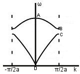
A. ka<<1, $\omega=\{\frac{2C(m_1+m_2)}{m_1m_2}\}^{\frac{1}{2}}$ , $\frac{B}{A}=\frac{-m_1}{m_2}$

m₁ and m₂ oscillate in antiphase and with different amplitudes.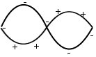

B. $ka=\frac{\pi}{2}$ , $\omega=\sqrt{\frac{2C}{m_2}}$ , $\frac{B}{A}=\infty$

Heavier atoms are stationary, lighter atoms oscillate.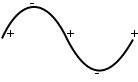

C. $ka=\frac{\pi}{2}$ , $\omega=\sqrt{\frac{2C}{m_1}}$ , $\frac{B}{A}=0$

Lighter atoms are stationary, heavier atoms oscillate.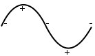

D. ka<<1, ω~v_sk, $latex \frac{B}{A}\simeq 1

Both masses oscillate in phases with the same amplitude.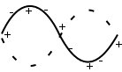

On the acoustic branch, atoms are in phase near D -> sound waves.

On the optic branch, atoms are in antiphase near A. There is an overall dipole moment so optical transitions can be excited.

In 3D: for p atoms in the basis, we have 3p equations of motion in 3D -> 3p branches of the dispersion curve. Three of these branches are acoustic modes (1 longitudinal, 2 transverse), leaving 3p-3 optic branches.

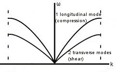
Since it is harder to shear than to compress, v_s is smaller for the transverse modes.

Lattice quantisation and normal modes: if a system is in a normal mode, all components of the system are oscillating at the same frequency. If the Hamilton of the system contains only harmonic terms, these modes are uncoupled.

Take a system with a purely harmonic potential so that the normal modes look like harmonic oscillators.

Energy levels $E=(n+\frac{1}{2})\bar{h}\omega$

$<E>=\frac{\sum_n (n+\frac{1}{2})\bar{h}\omega e^{\frac{-(n+\frac{1}{2})\bar{h}\omega}{kT}}}{\sum_n e^{\frac{-(n+\frac{1}{2})\bar{h}\omega}{kT}}}$

If we want to go ahead and work out these summations, then proceed as follows.

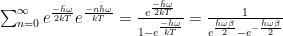
$\sum_{n=0}^{\infty}e^{\frac{-\bar{h}\omega}{2kT}} e^{\frac{-n\bar{h}\omega}{kT}} = \frac{ e^{\frac{-\bar{h}\omega}{2kT}}}{1- e^{\frac{-\bar{h}\omega}{kT}}} = \frac{1}{ e^{\frac{\bar{h}\omega\beta}{2}}- e^{-\frac{\bar{h}\omega\beta}{2}}}$

(geometric progression)

$\beta=\frac{1}{kT}$ as in thermodynamics.

$\sum_{n=0}^{\infty}(n+\frac{1}{2})\bar{h}\omega e^{\frac{-(n+\frac{1}{2})\bar{h}\omega}{kT}} = -\frac{d}{d\beta}(\frac{1}{ e^{\frac{\bar{h}\omega\beta}{2}}- e^{-\frac{\bar{h}\omega\beta}{2}}}) = \frac{\bar{h}\omega}{2}\frac{e^{\frac{\bar{h}\omega\beta}{2}}+ e^{-\frac{\bar{h}\omega\beta}{2}}}{ e^{\frac{\bar{h}\omega\beta}{2}}- e^{-\frac{\bar{h}\omega\beta}{2}}}$

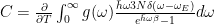
Lattice heat capacity: $C=\frac{\partial<E_{tot}>}{\partial T}$

$<E_{tot}>=\int_0^{\infty} \bar{h}\omega g(\omega)f(\omega)d\omega$

For phonons, $f(\omega)=\frac{1}{e^{\bar{h}\omega\beta}-1}$

$C=\frac{\partial}{\partial T}\int_0^{\infty}g(\omega)\frac{\bar{h}\omega}{e^{\bar{h}\omega\beta}-1}d\omega$

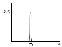
Einstein model: assume each atom is in an isolated potential at frequency ω_E. All atoms are at the same frequency, and each atom vibrates independently (no coupling).

$g(\omega)=3N\delta(\omega-\omega_E)$ (in 3D we have 3N oscillators)

$C=\frac{\partial}{\partial T}\int_0^{\infty}g(\omega)\frac{\bar{h}\omega3N\delta(\omega-\omega_E)}{e^{\bar{h}\omega\beta}-1}d\omega$

$C=\frac{\partial}{\partial T}\{\frac{3N\bar{h}\omega_E}{e^{\bar{h}\omega_E\beta}-1}\}$

$C=3N\bar{h}\omega_E(\frac{\bar{h}\omega_E}{kT^2})\frac{e^{\frac{\bar{h}\omega_E}{kT}}}{(e^{\frac{\bar{h}\omega_E}{kT}}-1)^2}$

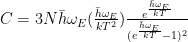
Define the Einstein temperature $\theta_E=\frac{\bar{h}\omega_E}{k}$

$C=3Nk(\frac{\theta_E}{T})^2\frac{e^{\frac{\theta_E}{T}}}{( e^{\frac{\theta_E}{T}-1^2})}$

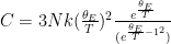
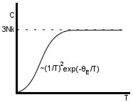
The Einstein model is not good for low temperature, although it does work fairly well at high temperature, where it tends to the classical result. Overall, though, this is not a good model- Einstein didn’t get it right all the time!

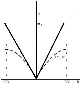
Debye model: approximate the dispersion curve as ω=v_sk all the way up to k=±π/a.

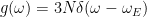
3N oscillators (still working in 3D)

$g(\omega)d\omega=3g(k)dk$

$g(\omega)=3g(k)\frac{dk}{d\omega}$

$g(\omega)=\frac{V}{(2\pi)^3}4\pi k^2\frac{dk}{d\omega}$

$g(\omega)=\frac{3V\omega^2}{2\pi^2v_s^3}$ for ω≤ ω_D

$g(\omega)=0$ otherwise

ω_D cut-off determined by 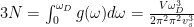$3N=\int_0^{\omega_D}g(\omega)d\omega=\frac{V\omega_D^3}{2\pi^2\pi^2v_s^3}$ (1)

Heat capacity

$C=\frac{\partial}{\partial T}\int_0^{\omega_D}\frac{3V\omega^2}{2\pi^2v_s^3}\frac{\bar{h}\omega}{e^{\frac{bar{h}\omega}{kT}}-1}d\omega$

Put $x=\frac{bar{h}\omega}{kT}$ and define the Debye temperature $\theta_D=\frac{\bar{h}\omega_D}{k}$

Now we can write

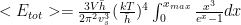
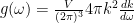
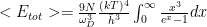
$<E_{tot}>=\frac{3V\bar{h}}{2\pi^2v_s^3}(\frac{kT}{\bar{h}})^4\int_0^{x_{max}}\frac{x^3}{e^x-1}dx$ where $x_{max}=\frac{\theta_D}{T}$

Substitute for v_s using (1) and tidy up to get

$<E_{tot}>=\frac{9N}{\omega_D^3}\frac{(kT)^4}{\bar{h}^3}\int_0^{x_{max}}\frac{x^3}{e^x-1}dx$

At low temperatures, x is large and upper states are unoccupied, so we can let the upper limit tend to infinity.

$<E_{tot}>=\frac{9N}{\omega_D^3}\frac{(kT)^4}{\bar{h}^3}\int_0^{\infty}\frac{x^3}{e^x-1}dx$

The integral is a standard one which we can look up to see that the answer is $\frac{\pi^4}{15}$

$<E_{tot}>=\frac{\pi^4}{15}\frac{9N}{\omega_D^3\bar{h}^3}(kT)^4$

$<E_{tot}>=\frac{3\pi^4}{5}nk\frac{T^4}{\theta_D^3}$

$C=\frac{12\pi^4}{5}nk\frac{T^3}{\theta_D^3}$

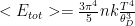
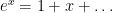
At high temperatures x is small, so we can expand e^x and ignore higher order terms.

$e^x=1+x+\ldots$

$<E_{tot}>=\frac{9N}{\omega_D^3}\frac{(kT)^4}{\bar{h}^3}\int_0^{x_{max}}\frac{x^3}{1+x-1}dx$

$<E_{tot}>=\frac{9N}{\omega_D^3}\frac{(kT)^4}{\bar{h}^3}\frac{x_{max}^3}{3}$

$<E_{tot}>=3NkT$

$C=3Nk=3R \textnormal{ per mole}$ (Dulong-Petit law)

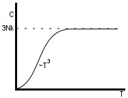
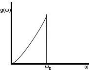
The Debye model is a good approximation at low ( $\sim\frac{\theta_D}{10}$ ) and high temperatures, but it is not very good for intermediate temperatures.

Actual density of states: as we know, the real dispersion relation has a lower ω_max than the one given by the Debye model- this means that g(ω) peaks earlier than in the Debye model.

Below this peak, $C\propto T^3$ as Debye says.

Considering transverse modes-

We would also see higher peaks if optic modes are present.

Density of states summary

Dimensions	g(k)	g(ω)		Heat capacity
Dimensions	g(k)	electrons $\frac{\bar{h}^2k^2}{2m}$	photons/phonons $\bar{h}ck$ / $\bar{h}v_sk$	low temp due to phonons	due to electrons
1	const	~ε^-1/2	const	~T	~T
2	~k	const	~ε	~T²	~T
3	~k²	~ε^1/2	~ε²	~T³	~T

Physics Made Easy